In some of our past blogs, we have discussed how SQL Server Statistics are created, automatically maintained & updated demonstrating how the different computations of the histogram are done. With that said, today’s blog will be dealing with how this computed data is used by the SQL optimizer for Cardinality Estimation.
Histogram includes a lot of data such as Density Factor, RANGE_HI_KEYS, RANGE_ROWS, EQ_ROWS, DISTINCT_ROWS, and AVG_RANGE_ROWS.
The prime focus of this blog will be on RANGE_ROWS & EQ_ROWS.
We will be using AdventureWorks2008 for this demo.
The table SalesOrderHeader contains a TotalDue column (as shown below). This column comprises a variety of values ranging from a single-digit to multiple digits.
SELECT * FROM Sales.SalesOrderHeader

Now, let’s create statistics on TotalDue and then view the histogram using the DBCC SHOW_STATISTICS command.
CREATE STATISTICS TotalDue ON Sales.SalesOrderHeader(TotalDue)
GO
DBCC SHOW_STATISTICS (N'Sales.SalesOrderHeader', TotalDue)
GO

The histogram data is comprised of all the different columns mentioned earlier. For now, we will look into the most basic column EQ_ROWS.
On selecting a particular value from the boundaries of the histogram (RANGE_HI_KEY column), the EQ_ROWS tells the optimizer the exact number of rows in TotalDue column that match the value. But, in the case of a value that is not an exact match, but is present in-between two distinct values in the RANGE_HI_KEY column, it returns the AVG_RANGE_ROWS value instead. This is where the computed data from the histogram comes into play.
On selecting a value between 30.6859 & 32.0229, the optimizer always returns a value of 4.6, as computed in the AVG_RANGE_ROWS column.

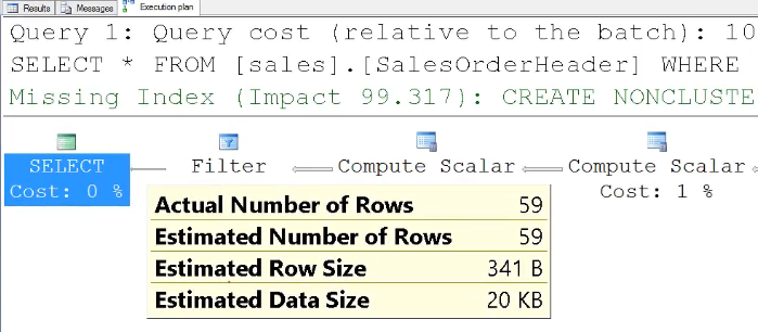
The query shown below returns 59 rows having a value of 32.0229, which is the same as the value provided to us in the EQ_ROWS histogram statistics as seen earlier.
SELECT * FROM Sales.SalesOrderHeader
WHERE TotalDue = 32.0229
In the Execution Plan, upon hovering over the Filter operator, it is seen that the Actual Number of Rows & Estimated Number of Rows is the same. This is considered to be 100% or perfect Cardinality Estimation.

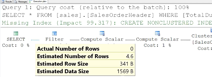
Changing the value at the WHERE clause to 31, the same query returns an empty result set since there are no values in the RANGE_HI_KEY that is an exact match.
SELECT * FROM Sales.SalesOrderHeader
WHERE TotalDue = 31
However, the Execution Plan shows an estimation of 4.6, similar to the computed value in the AVG_RANGE_ROWS column.

This operation can be performed with other values that do not directly reside in the RANGE_HI_KEY column, only to obtain similar results. This demonstrates how Statistics are used by the optimizer for Cardinality Estimation.
